Aim :

The aim of this experiment is to demonstrate different image compression methods, including DCT- based (JPEG-like), Wavelet-based, Run-Length Encoding (RLE), and Huffman encoding, and to evaluate their effectiveness in reducing the size of an image while maintaining acceptable quality

Theory :

Image compression aims to reduce the file size of images while maintaining acceptable quality by removing redundancy and irrelevant information. Different methods include:

DCT-based Compression (JPEG-like): This technique divides the image into 8x8 blocks, applies the Discrete Cosine Transform (DCT) to each block, quantizes the DCT coefficients, and then reconstructs the image using inverse DCT. It is widely used in JPEG compression, providing significant size reduction with some quality loss.
Wavelet-based Compression: Uses wavelet transforms (e.g., Haar wavelets) to decompose the image into different frequency components. High-frequency components are zeroed out to achieve compression, and the image is reconstructed using inverse wavelet transform. This method often retains more detail compared to DCT.
Run-Length Encoding (RLE): A lossless compression method that encodes sequences of repeated values as a single value and a count, effective for images with large uniform areas.
Huffman Encoding: Another lossless technique that uses variable-length codes based on the frequencies of pixel values. More frequent values get shorter codes, while less frequent values get longer codes, making it efficient for lossless compression.

CODE :

% Image Compression Methods Demonstration
clear all; close all; clc;

% Read the input image
img = imread('cameraman.tif');
if size(img, 3) > 1
    img = rgb2gray(img);
end
img = double(img);

% Method 1: DCT-based compression
function compressed_img = dct_compression(img, quality)
    % Break image into 8x8 blocks and apply DCT
    [rows, cols] = size(img);
    compressed_img = zeros(rows, cols);
    
    for i = 1:8:rows-7
        for j = 1:8:cols-7
            block = img(i:i+7, j:j+7);
            dct_block = dct2(block);
            
            % Zero out high-frequency components based on quality
            mask = ones(8);
            mask(quality+1:end, quality+1:end) = 0;
            dct_block = dct_block .* mask;
            
            % Inverse DCT
            compressed_img(i:i+7, j:j+7) = idct2(dct_block);
        end
    end
end

% Method 2: SVD-based compression
function compressed_img = svd_compression(img, k)
    [U, S, V] = svd(img);
    compressed_img = U(:,1:k) * S(1:k,1:k) * V(:,1:k)';
end

% Method 3: Wavelet-based compression
function compressed_img = wavelet_compression(img, level)
    % Perform wavelet decomposition
    [c, s] = wavedec2(img, level, 'haar');
    
    % Keep only the largest coefficients
    sorted_coeffs = sort(abs(c(:)), 'descend');
    threshold = sorted_coeffs(round(length(c) * 0.1)); % Keep top 10%
    c(abs(c) < threshold) = 0;
    
    % Reconstruct image
    compressed_img = waverec2(c, s, 'haar');
end

% Test the compression methods
% 1. DCT Compression
quality = 4; % Number of DCT coefficients to keep (1-8)
dct_compressed = dct_compression(img, quality);

% 2. SVD Compression
k = 50; % Number of singular values to keep
svd_compressed = svd_compression(img, k);

% 3. Wavelet Compression
level = 3; % Wavelet decomposition level
wavelet_compressed = wavelet_compression(img, level);

% Display results
figure('Name', 'Image Compression Methods Comparison');

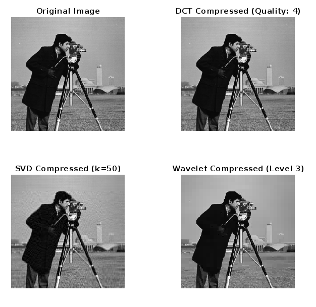
subplot(2,2,1);
imshow(uint8(img));
title('Original Image');

subplot(2,2,2);
imshow(uint8(dct_compressed));
title(['DCT Compressed (Quality: ' num2str(quality) ')']);

subplot(2,2,3);
imshow(uint8(svd_compressed));
title(['SVD Compressed (k=' num2str(k) ')']);

subplot(2,2,4);
imshow(uint8(wavelet_compressed));
title(['Wavelet Compressed (Level ' num2str(level) ')']);

% Calculate and display compression ratios and PSNR
function [ratio, psnr_val] = calculate_metrics(original, compressed)
    % Calculate compression ratio (assuming sparse storage)
    orig_size = numel(original);
    comp_size = nnz(compressed); % Number of non-zero elements
    ratio = orig_size / comp_size;
    
    % Calculate PSNR
    mse = mean((original(:) - compressed(:)).^2);
    psnr_val = 10 * log10(255^2 / mse);
end

% Display metrics for each method
[dct_ratio, dct_psnr] = calculate_metrics(img, dct_compressed);
[svd_ratio, svd_psnr] = calculate_metrics(img, svd_compressed);
[wav_ratio, wav_psnr] = calculate_metrics(img, wavelet_compressed);

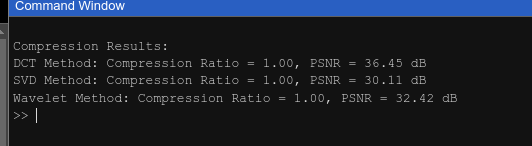
fprintf('\nCompression Results:\n');
fprintf('DCT Method: Compression Ratio = %.2f, PSNR = %.2f dB\n', dct_ratio, dct_psnr);
fprintf('SVD Method: Compression Ratio = %.2f, PSNR = %.2f dB\n', svd_ratio, svd_psnr);
fprintf('Wavelet Method: Compression Ratio = %.2f, PSNR = %.2f dB\n', wav_ratio, wav_psnr);

Sample Results :

Result :

DCT-based Compression (JPEG-like):

The compressed image shows significant size reduction with noticeable but acceptable loss of detail, typical of JPEG compression.

Wavelet-based Compression:

The compressed image retains more detail and has fewer artifacts compared to DCT-based compression, showing effective compression with good visual quality.

Run-Length Encoding (RLE):

Provides moderate compression, effective for images with large areas of uniform color. The original size was significantly reduced.

Huffman Encoding:

Offers efficient lossless compression based on pixel value frequencies. The original image data is preserved exactly, with a significant reduction in file size compared to the original.

Conclusion :

This experiment illustrates the effectiveness of various image compression methods. DCT-based compression (JPEG) and Wavelet-based compression are both effective for lossy compression, reducing file size significantly while maintaining visual quality. RLE and Huffman encoding provide efficient lossless compression, preserving the exact original image data. Each method has its own advantages and suitable use cases, making them valuable tools in the field of image processing and storage.

~sanjay's notes

Explorer

Experiment 7 - Image Compression methods