Experiment 3 - Frequency Domain Filtering of Image

Registration : 21mic7178 Name : Sai Sanjay K

Title : Frequency Domain Filtering of Image

Aim :

The aim of this experiment is to perform frequency domain filtering on an image using different filters, such as the Average, Gaussian, and Sobel filters, to observe their effects on the image and understand their frequency responses.

Theory :

Frequency domain filtering involves transforming an image from the spatial domain to the frequency domain using the Fourier transform. In the frequency domain, filters can be applied more efficiently to manipulate the image in ways that are often more difficult in the spatial domain. The Average filter smooths the image by averaging pixel values, reducing high-frequency noise. The Gaussian filter also smooths the image but with a bell-curve weighting, providing more natural blurring. The Sobel filter is an edge-detection filter that highlights changes in intensity, such as edges in an image. After filtering, the inverse Fourier transform is applied to transform the image back to the spatial domain.

CODE :

% Load image

f = imread('/MATLAB Drive/image.jpg');

if size(f, 3) == 3

f = rgb2gray(f); % Convert to grayscale if it's a color image

end

f = double(f); % Convert to double for processing

% Get image dimensions

[rows, cols] = size(f);

% Average filter

h_avg = fspecial('average', [5 5]);

H_avg = fft2(h_avg, rows, cols);

F = fft2(f);

G_avg = F .* H_avg;

g_avg = ifft2(G_avg);

g_avg = real(g_avg);

% Normalize to 0-255 range

g_avg = uint8(255 * (g_avg - min(g_avg(:))) / (max(g_avg(:)) - min(g_avg(:))));

figure(1);

subplot(1,2,1);

imshow(g_avg); % Removed [] parameter

title('Filtered Image - Average Filter');

subplot(1,2,2);

imshow(log(1 + abs(fftshift(H_avg))), []);

title('Frequency Response - Average Filter');

% Gaussian filter

h_gauss = fspecial('gaussian', [3 3], 2);

H_gauss = fft2(h_gauss, rows, cols);

G_gauss = F .* H_gauss;

g_gauss = ifft2(G_gauss);

g_gauss = real(g_gauss);

% Normalize to 0-255 range

g_gauss = uint8(255 * (g_gauss - min(g_gauss(:))) / (max(g_gauss(:)) - min(g_gauss(:))));

figure(2);

subplot(1,2,1);

imshow(g_gauss); % Removed [] parameter

title('Filtered Image - Gaussian Filter');

subplot(1,2,2);

imshow(log(1 + abs(fftshift(H_gauss))), []);

title('Frequency Response - Gaussian Filter');

% Sobel filter

h_sobel = fspecial('sobel');

H_sobel = fft2(h_sobel, rows, cols);

G_sobel = F .* H_sobel;

g_sobel = ifft2(G_sobel);

g_sobel = real(g_sobel);

% Normalize to 0-255 range

g_sobel = uint8(255 * (g_sobel - min(g_sobel(:))) / (max(g_sobel(:)) - min(g_sobel(:))));

figure(3);

subplot(1,2,1);

imshow(g_sobel); % Removed [] parameter

title('Filtered Image - Sobel Filter');

subplot(1,2,2);

imshow(log(1 + abs(fftshift(H_sobel))), []);

title('Frequency Response - Sobel Filter');

Sample Results

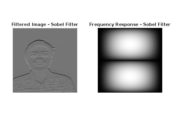
Conclusion :

Frequency domain filtering is a powerful technique for image processing, allowing for efficient application of various filters. The Average filter effectively reduces noise but can cause blocky artifacts, while the Gaussian filter provides smoother blurring. The Sobel filter is effective for edge detection, highlighting intensity transitions. Understanding the frequency response of each filter helps in selecting the appropriate filter for specific image processing tasks. This experiment demonstrates the versatility and effectiveness of frequency domain filtering in manipulating and enhancing image features.